
 |
Turbulence Modeling Resource |
Note that the use of overbars and hats, indicating time averaging and density-weighted averaging
(described on this page) is not always followed throughout the
rest of the website. Often, they are dropped for convenience.
Implementing Turbulence Models into the Compressible RANS Equations
There are many technical papers and texts that derive and/or
describe the compressible Reynolds-averaged Navier-Stokes equations (also termed the Favre-averaged
Navier-Stokes equations). See, for example,
(1) Gatski, T. B. and Bonnet, J.-P., "Compressibility, Turbulence and High Speed Flow,"
2009, Elsevier, Amsterdam, (2) Wilcox, D. C., "Turbulence Modeling for CFD," 2006, DCW Industries, La Canada, CA, or
(3) Hirsch, C., "Numerical Computation of Internal and External Flows, Vol. 2," 1990, John Wiley & Sons,
Chichester.
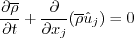
The equations can be written as follows:
where
and the viscous stress tensor is:
Note that the Reynolds stress term
where
The equation of state is:
where k is the local turbulent kinetic energy (the kinetic energy of the fluctuating field):
Most turbulence modeling focuses on the Reynolds stress terms
( where Less attention is typically given to the other terms that need to be modeled.
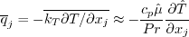
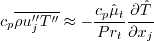
Most commonly, a Reynolds analogy is used to model the turbulent heat flux:
where Prt is a "turbulent Prandtl number," often taken to be constant (e.g.,
around 0.9 for air).
Ideal gas relations are typically used to resolve the heat capacity at constant pressure (cp);
if required, the specific gas constant for air is usually taken as 287.058 J/(kgK).
The terms associated with molecular diffusion and turbulent transport
in the energy equation are modeled different ways (often lumped together). For example, one model is:
where Return to: Turbulence Modeling Resource Home Page
Recent significant updates:
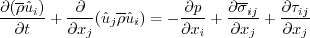


 is defined in the literature both as shown here, as well as
with the opposite sign, and sometimes without the density included in the definition.
(This different terminology does not matter, as long as consistency is maintained throughout the derivation.)
The term cp is the heat capacity at constant pressure, and Pr is the Prandtl number (e.g.,
around 0.72 for air).
On this page the overbar indicates conventional time-average mean, with the averaging time scale assumed to be
long compared to turbulent fluctuations, and short compared to unsteadiness in the mean flow.
The hat here represents the Favre (density-weighted) average:
is defined in the literature both as shown here, as well as
with the opposite sign, and sometimes without the density included in the definition.
(This different terminology does not matter, as long as consistency is maintained throughout the derivation.)
The term cp is the heat capacity at constant pressure, and Pr is the Prandtl number (e.g.,
around 0.72 for air).
On this page the overbar indicates conventional time-average mean, with the averaging time scale assumed to be
long compared to turbulent fluctuations, and short compared to unsteadiness in the mean flow.
The hat here represents the Favre (density-weighted) average:
 .
Note that
.
Note that 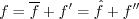 .
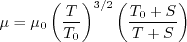
The dynamic viscosity,
.
The dynamic viscosity,  , is
often computed using
Sutherland's Law, which gives a relationship between the dynamic viscosity
and the temperature of an ideal gas (See White, F. M., "Viscous Fluid Flow," McGraw Hill, New York, 1974, p. 28).
In Sutherland's Law, the local value of dynamic viscosity is determined by plugging the local value of temperature
(T) into the following formula:
, is
often computed using
Sutherland's Law, which gives a relationship between the dynamic viscosity
and the temperature of an ideal gas (See White, F. M., "Viscous Fluid Flow," McGraw Hill, New York, 1974, p. 28).
In Sutherland's Law, the local value of dynamic viscosity is determined by plugging the local value of temperature
(T) into the following formula:
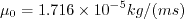 ,
,
 , and
, and
 .
The same formula can be found online
(with temperature constants given in degrees K and some small conversion differences).
.
The same formula can be found online
(with temperature constants given in degrees K and some small conversion differences).
![\overline p = (\gamma - 1)[\overline\rho \hat E -
\frac{1}{2}\overline\rho ( \hat u^2 + \hat v^2 + \hat w^2) - \overline\rho k]](implementrans_eqns/img10.png)
![k = [(\hat {u_i''})^2 + (\hat {v_i''})^2 + (\hat {w_i''})^2]/2](implementrans_eqns/img18.png) .
(The k term is sometimes ignored in the equation of state for non-supersonic speed flows.)
The heat capacity ratio (
.
(The k term is sometimes ignored in the equation of state for non-supersonic speed flows.)
The heat capacity ratio ( ) is typically
taken as constant at 1.4 for air.
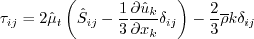
The following terms in the Favre-averaged equations need to be modeled:
) is typically
taken as constant at 1.4 for air.
The following terms in the Favre-averaged equations need to be modeled:


 ).
These are either solved directly (as in full second-moment Reynolds stress models) or
defined via a constitutive relation for simpler models.
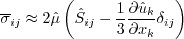
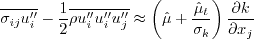
For example, the common Boussinesq approximation is:
).
These are either solved directly (as in full second-moment Reynolds stress models) or
defined via a constitutive relation for simpler models.
For example, the common Boussinesq approximation is:
 , and
, and
 is the eddy viscosity
obtained by the turbulence model.
(In the equation above, the
is the eddy viscosity
obtained by the turbulence model.
(In the equation above, the  term is sometimes ignored for non-supersonic
speed flows, and the second term in parentheses is identically zero for incompressible flows.)
term is sometimes ignored for non-supersonic
speed flows, and the second term in parentheses is identically zero for incompressible flows.)
 (which is sometimes shown like this, in the denominator, and sometimes in
the numerator with its value adjusted accordingly) is a coefficient associated with the modeling equation for k.
This expression in the energy equation is also sometimes neglected.
(which is sometimes shown like this, in the denominator, and sometimes in
the numerator with its value adjusted accordingly) is a coefficient associated with the modeling equation for k.
This expression in the energy equation is also sometimes neglected.
07/10/2021 - mentioned that sigma_k sometimes is written in the numerator
01/10/2017 - added mention of gamma and specific gas constant for air
08/22/2013 - added equation for Sutherland's Law
07/08/2013 - fixed typo in energy equation
Page Curators: Christopher Rumsey,
Ethan Vogel,
Clark Pederson
Clark Pederson
Last Updated: 10/10/2024